Objective – By the end of this lecture, the student should be able to perform a Fourier analysis on a circuit.
Sec. 7-1 Fourier analysis
Fourier analysis is useful when the harmonic distortion of the circuit is to be determine. For this part of the lecture, we will be using a simple full wave rectifier circuit, refer to fig. 7-1. This circuit takes a voltage source, a sinewave and output a DC voltage. This circuit does yield a significant amount of harmonic distortion.
|
|
| Fig. 7-1 – Full wave rectifier circuit |
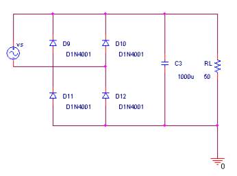
- Create the circuit as shown in fig. 7-1
- Change the reference for the VSIN to Vs
- Set the VAMPL to 35V
- Set the Freq to 60 Hz
- Change the reference for the resistor to RL
- Create a new simulation profile
- Select Transient Analysis as the analysis type
- Type in 50ms for the Run Time
- Type in 1ms for the Maximum Step Time
- Click on Output File Option
- Check the Perform Fourier Analysis option
- Type in 60 for the Center Frequency
This is the frequency of the input and output signal - Type in 19 for the Number of Harmonics
This specify the number of harmonics to calculate - Type in I(rL) for the Output Variable
This specify to perform the FFT on the current through the load resistance - Click OK
- Click OK
- Run the simulation
After the simulation is run, go to the Probe window and click on View/Output File. The following is an except from the output file:
DC COMPONENT =  -5.959139E-01

HARMONIC   FREQUENCY    FOURIER    NORMALIZED    PHASE    NORMALIZED

  NO         (HZ)     COMPONENT    COMPONENT    (DEG)       PHASE(DEG)

 1    	 6.000E+01    6.197E-02    1.000E+00    1.178E+02    0.000E+00

 2     	 1.200E+02    2.926E-02    4.721E-01    5.142E+01   -6.635E+01

 3       1.800E+02    1.759E-02    2.838E-01   -1.324E+01   -1.310E+02

 4       2.400E+02    1.133E-02    1.829E-01   -7.686E+01   -1.946E+02

 5       3.000E+02    7.447E-03    1.202E-01   -1.394E+02   -2.572E+02

 6       3.600E+02    4.905E-03    7.915E-02    1.597E+02    4.188E+01

 7       4.200E+02    3.233E-03    5.217E-02    1.016E+02   -1.613E+01

 8       4.800E+02    2.154E-03    3.476E-02    4.789E+01   -6.987E+01

 9       5.400E+02    1.488E-03    2.402E-02   -1.686E+00   -1.195E+02

10       6.000E+02    1.088E-03    1.756E-02   -4.953E+01   -1.673E+02

11       6.600E+02    8.406E-04    1.357E-02   -9.944E+01   -2.172E+02

12       7.200E+02    6.677E-04    1.078E-02   -1.533E+02   -2.710E+02

13       7.800E+02    5.400E-04    8.715E-03    1.499E+02    3.216E+01

14       8.400E+02    4.340E-04    7.004E-03    9.303E+01   -2.474E+01

15       9.000E+02    3.479E-04    5.615E-03    3.830E+01   -7.946E+01

16       9.600E+02    2.676E-04    4.318E-03   -1.718E+01   -1.350E+02

17       1.020E+03    2.079E-04    3.355E-03   -7.627E+01   -1.940E+02

18       1.080E+03    1.569E-04    2.533E-03   -1.390E+02   -2.567E+02

19       1.140E+03    1.329E-04    2.145E-03    1.519E+02    3.412E+01

		TOTAL HARMONIC DISTORTION =   6.024097E+01 PERCENT
The output listing show the DC component, or the fundamental frequency, it also shows the total harmonic distortion, or THD. This listing is quite useful, but to really see the result clearing, the harmonics should be plotted. PSpice does not do this, so the data should be exported to an external application such as MS Excel and graphed.
Sec. 7.2 Exporting data to Excel
For this part of the lecture, we will be using the program MS Excel to plot the harmonics plot.
- Select the listing from the output file, and click on Edit/Copy
Choose only the part that’s relevant to the data, refer to fig. 7-2. - Open up the program Notepad, and select Edit/Paste, refer to
fig. 7-2
Notepad can be access by clicking Start/Programs/Accessories/Notepad
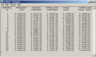
Fig. 7-2 – Notepad window
- Save the file with a .txt extension
- Open up the saved file in Excel.
- Once the file is open, Excel will present the text wizard import
dialog box, refer to fig. 7-3
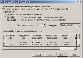
Fig. 7-3 – Excel text import wizard option dialog box step one
- In the option, select Delimited
- Click Next
- Select Space under the Delimited field
- This will put each data between spaces in its own cell
- Click Finish
- From the Excel window, click on a new column and type in Norm Mag
- Click on a cell below Norm Mag.
This column will be the normalize magnitude with respect to the first harmonics. - Type in the formaula =c4/$c$4This formula divides the first harmonics into the subsequent harmonics. The $ sign is an absolute addressing.
- Copy the equation from this cell and paste it to the following cell,
refer to fig. 7-4
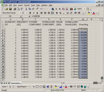
Fig. 7-4 – Formula pasted into cells.
- Create a graph using the Chart Wizard
- Select the Norm Mag column and the Harmonic No column
- Select Column for the Chart Type
The chart you get should be similar to fig. 7-5.
With this plot, it is easy to see the amount of distortion each harmonics contribute.
*Note – I am assuming the students have sufficient knowledge in using Excel, so I won’t go into details on using Excel*
 |
| Fig. 7-5 – Harmonic plot |
Sec. 7.3 Importing data into PSpice
There are ways to import data into PSpice so it could be simulated concurrently with the PSpice circuit. The easiest way I found to do this is to using the PWL (Piecewise Linear model). The PWL can either be a voltage source or a current source. The PWL have a few parts in which to import the data; one is to enter the data in manually; the other is to specify a data file.
The data file that the PWL will accept can be any data file as long as it’s in CSV format. The data file has to have two column data with the first column being the second and the second column being either the voltage or current. Between the two data, it has to be separate by a comma. A sample format would be as follow:
0,35
0.01,34
0.015,31
This would then be saved into a file and call from PSpice.
To call the file in PSpice, the best part to use is the VPWL_FILE located in the source library.
Sec. 7.4 Using PWL to create a one shot pulse wave
Technique 1
- Create the circuit in fig. 7-6
Fig. 7-6 – One shot pulse wave
- For the voltage source, use the part call VPWL in the source library
- Double click on the VPWL to access the data sheet
- For T1 type in 0
- For V1 type in 0
- For T2 type in 0.01
- For V2 type in 0
- For T3 type in 0.010001
- For V3 type in 5
- For T4 type in 0.02
- For T5 type in 0.020001
- For V5 type in 0
- Create a transient analysis
- Plot the voltage waveform for the VPWL, the waveform should look like fig. 7-7
|
|
|
Fig. 7-7 – Single shot pulse using PWL |
Technique 2
- Open up Notepad
- Type in the following values:
0,0
0.01,0
0.010001,5
0.02,5
0.02001,0 - Save the file as one_shot.txt
PSpice does not allow file with spaces, so an underscore should be used to separate the words for the file name. - Create the circuit in fig. 7-8
- For the voltage source use VPWL_FILE
- Double click on the <file> near the part
- Type in one_shot.txt
*NOTE – Make sure that one_shot.txt is located in the same folder as the PSpice file* - Create a transient analysis for 50ms
- Run the simulation
- Add a trace to plot he voltage of the VPWL_FILE
The plot should be the same as fig. 7-7.
The PWL is also useful if an uncommon signal need to be modeled or an almost perfect impulse function.
|
|
| Fig. 7-8 –One shot pulse using VPWL_FILE |